6 线性降维PCA[Perform linear dimensional reduction]
在Seurat中,不是直接对所有细胞进行聚类分析,而是首先进行PCA主成分分析,然后挑选贡献量最大的几个主成分,用挑选出的主成分的值来进行聚类分析
In Seurat, instead of directly performing cluster analysis on all cells, first perform PCA principal component analysis, then select the few principal components with the largest contribution, and use the selected principal component values for cluster analysis.
6.1 P-PCA结果[PCA result]
PCA结果[PCA result]
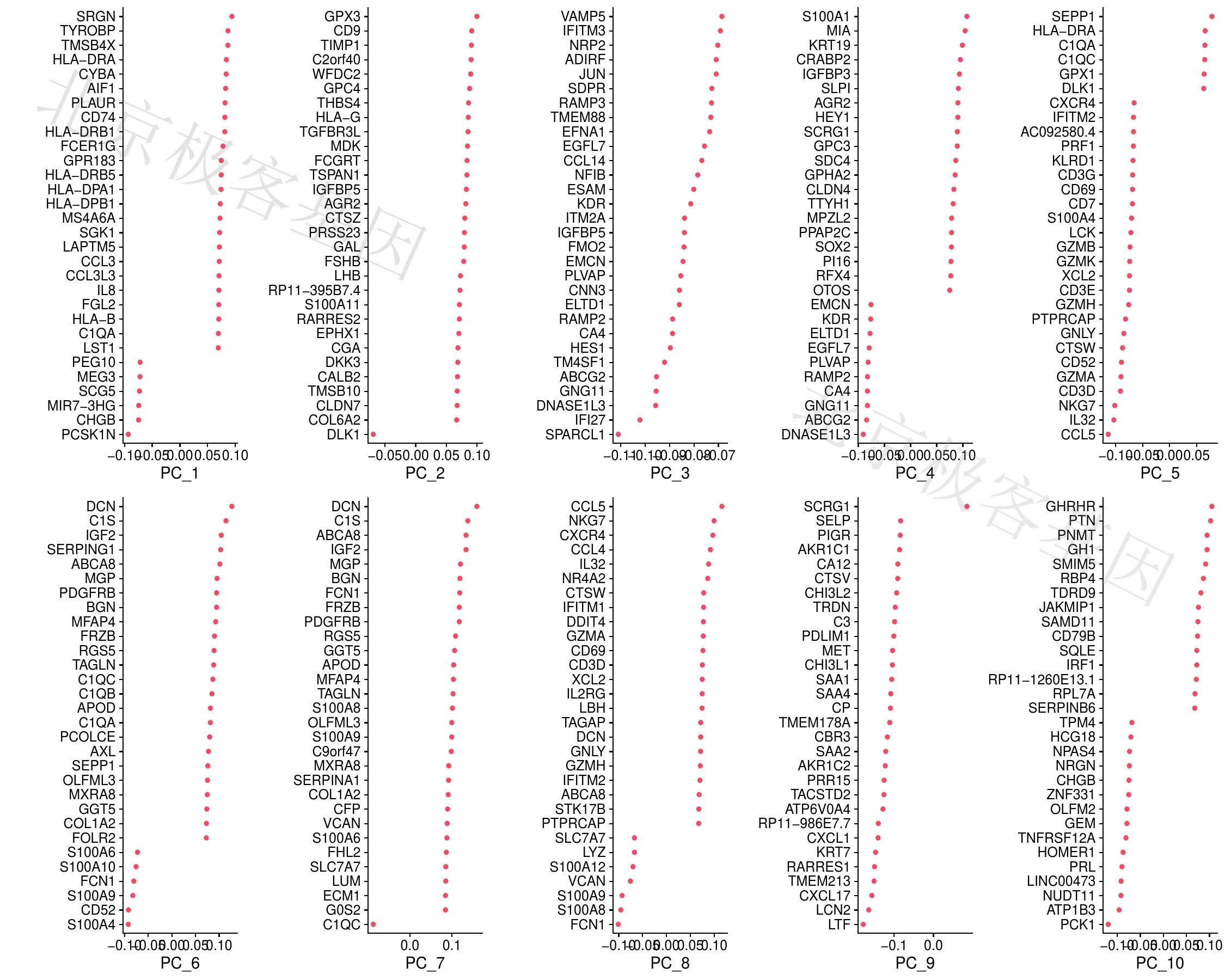
Figure 6.1: P-PCA result
PDF 文件 : P-VizDimLoadings.jpg
不同主成分的关系[Principal component relationship]
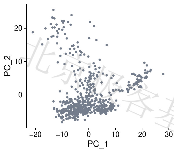
Figure 6.2: P-PCA relationship
PDF 文件 : P-DimPlot.jpg
主成分热图[Principal component heatmap]
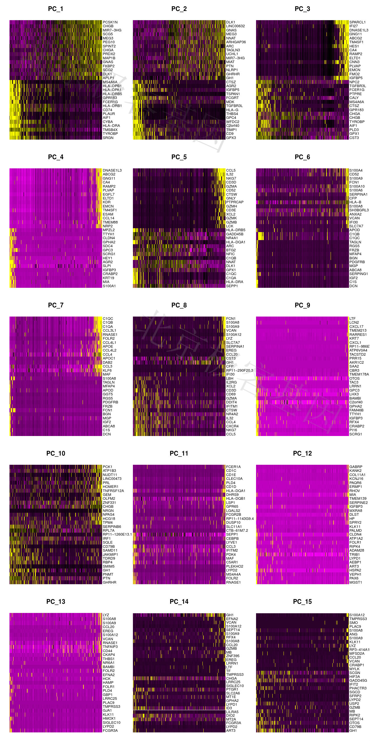
Figure 6.3: P-Main source of heterogeneity
PDF 文件 : P-DimHeatmap.jpg
鉴定数据集的可用维度[Determine statistically significant principal components]
分布图[Distribution]
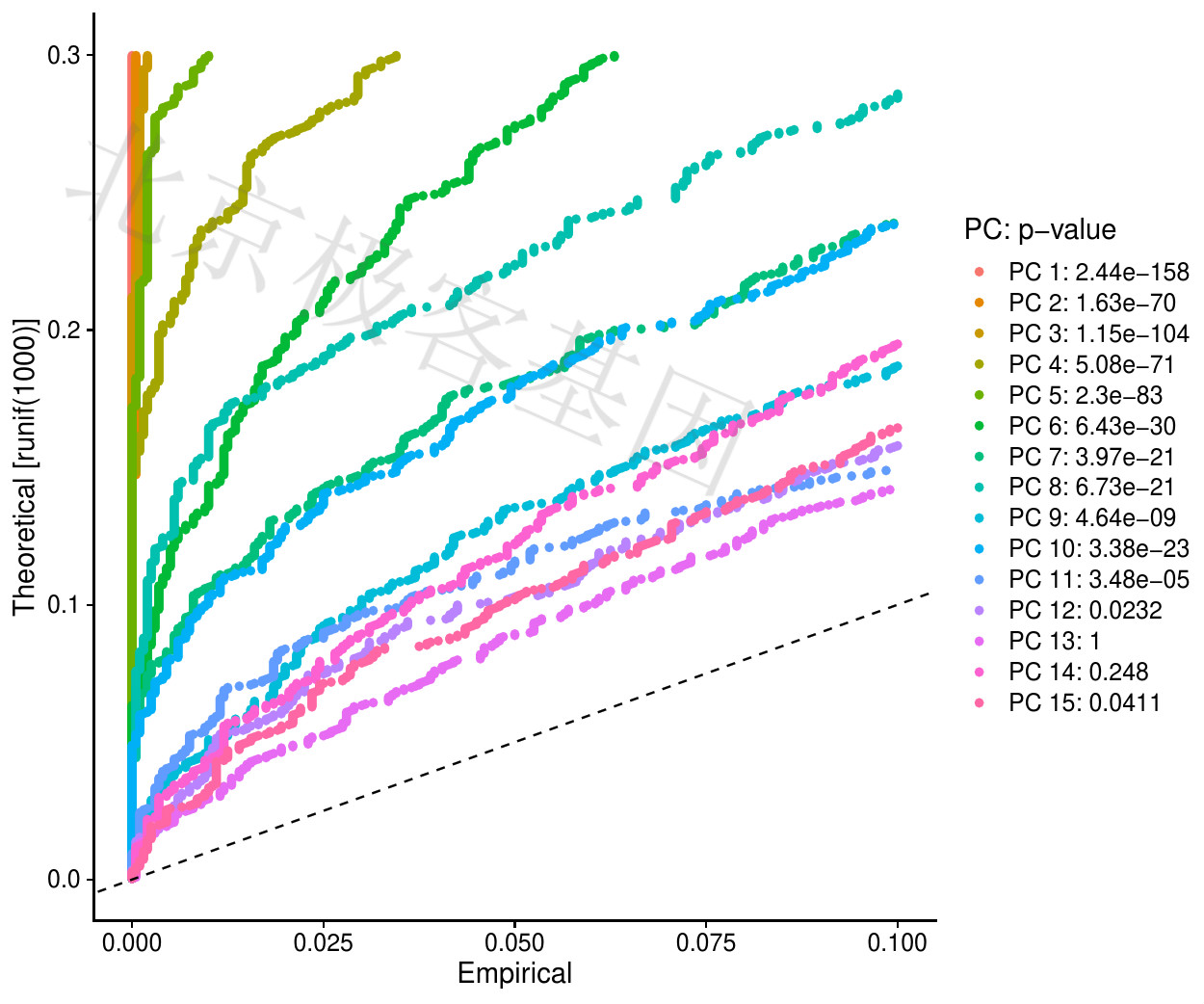
Figure 6.4: P-PCA result
PDF 文件 : P-main_pc1.jpg
图例[Figure legends]
比较每个PC的p值分布和均匀分布(虚线)。“重要的”PC将显示具有低p值的特征的强烈丰富(虚线上方的实线)。在这种情况下,看起来在前10-12个PC之后,重要性急剧下降。
Compare the p-value distribution and the uniform distribution (dashed line) for each PC. “Important” PCs will show a strong abundance of features with low p-values (solid lines above the dotted line). In this case, it looks like the importance drops sharply after the first 10-12 PCs.
肘图
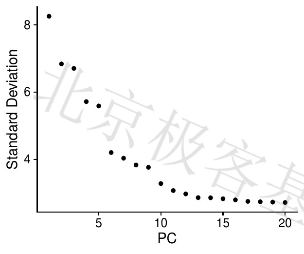
Figure 6.5: P-PCA result
PDF 文件 : P-main_pc1.jpg
图例[Figure legends]
基于每个(ElbowPlot函数)解释的方差百分比对主成分进行排序。在这个例子中,我们可以观察PC9-10周围的“肘部”,这表明大多数真实信号都是在前10PC中捕获的。
Sort the principal components based on the percentage of variance explained by each (ElbowPlot function). In this example, we can observe the “elbows” around PC9-10, which indicates that most of the real signals were captured in the top 10PCs.
6.2 T-PCA结果[PCA result]
PCA结果[PCA result]
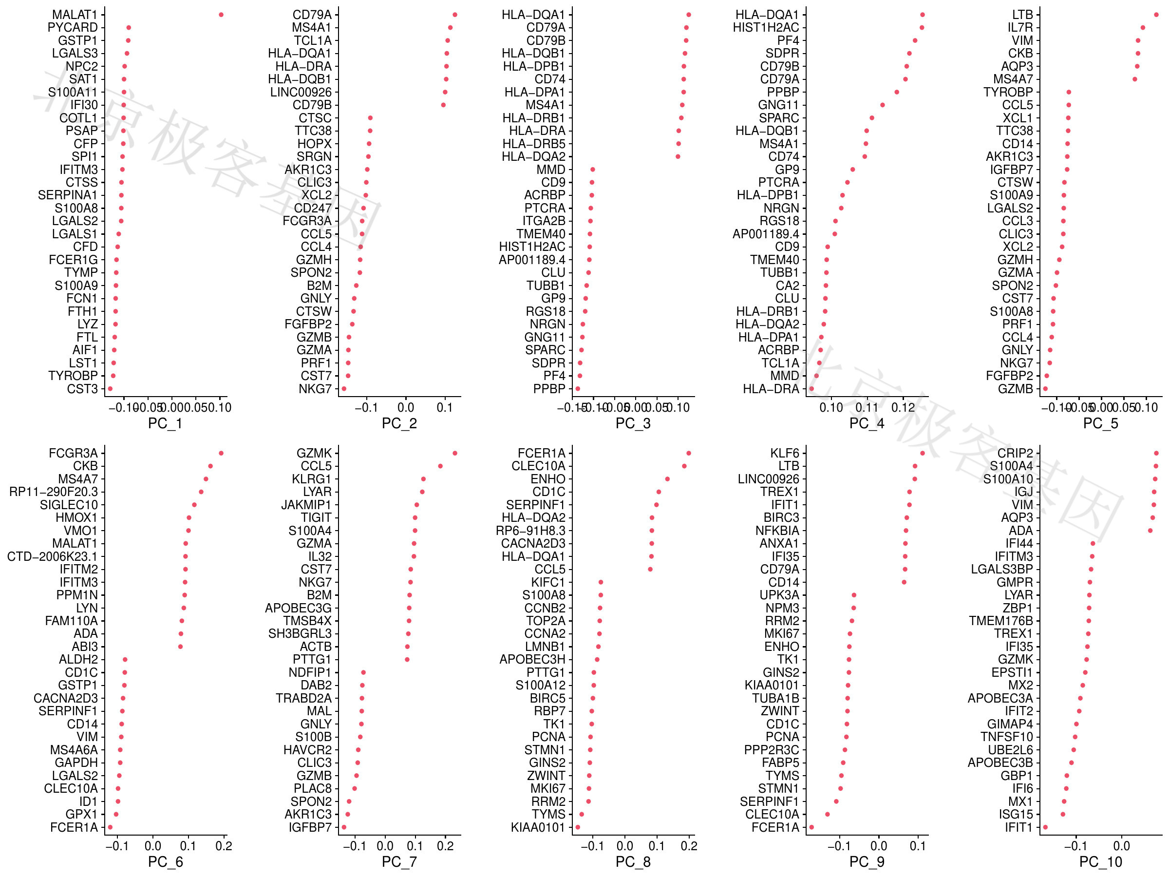
Figure 6.6: T-PCA result
PDF 文件 : T-VizDimLoadings.jpg
不同主成分的关系[Principal component relationship]
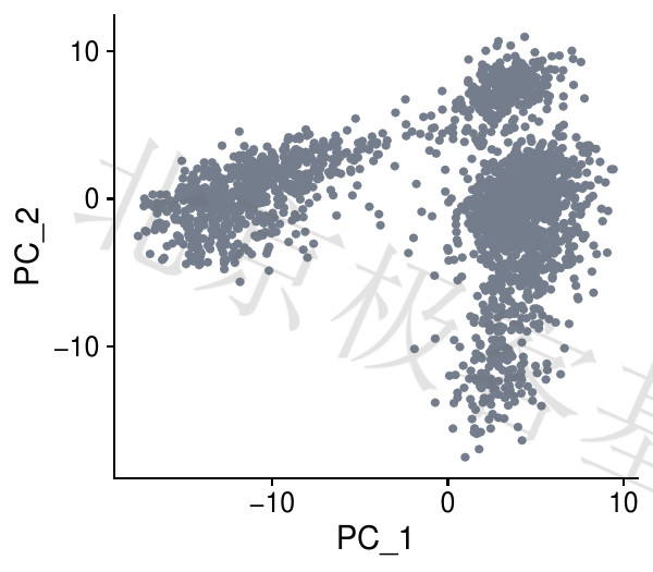
Figure 6.7: T-PCA relationship
PDF 文件 : T-DimPlot.jpg
主成分热图[Principal component heatmap]
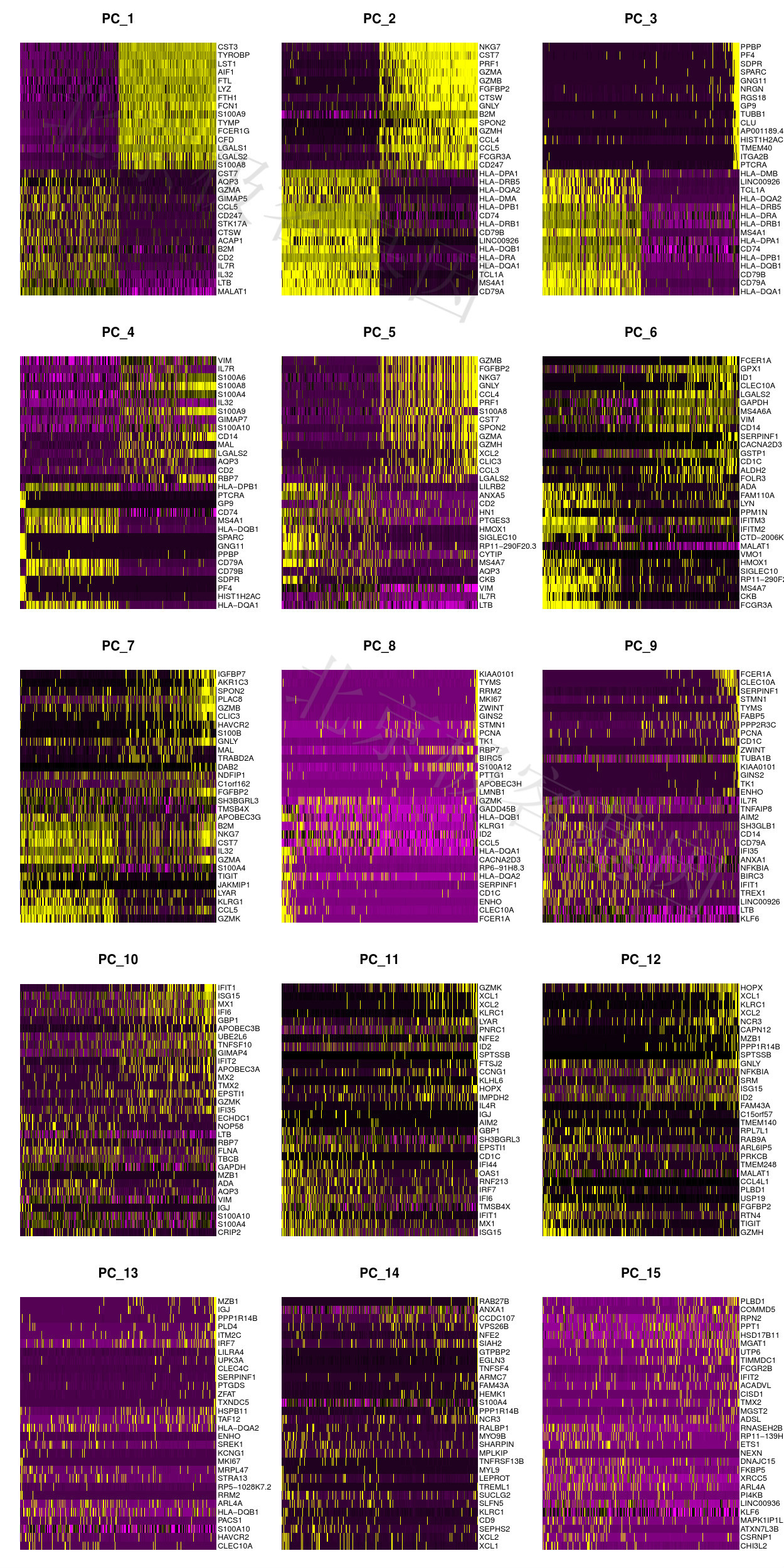
Figure 6.8: T-Main source of heterogeneity
PDF 文件 : T-DimHeatmap.jpg
鉴定数据集的可用维度[Determine statistically significant principal components]
分布图[Distribution]
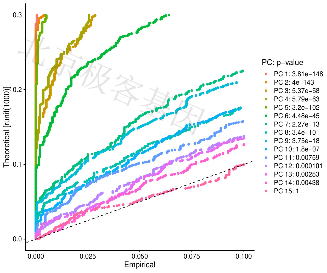
Figure 6.9: T-PCA result
PDF 文件 : T-main_pc1.jpg
图例[Figure legends]
比较每个PC的p值分布和均匀分布(虚线)。“重要的”PC将显示具有低p值的特征的强烈丰富(虚线上方的实线)。在这种情况下,看起来在前10-12个PC之后,重要性急剧下降。
Compare the p-value distribution and the uniform distribution (dashed line) for each PC. “Important” PCs will show a strong abundance of features with low p-values (solid lines above the dotted line). In this case, it looks like the importance drops sharply after the first 10-12 PCs.
肘图
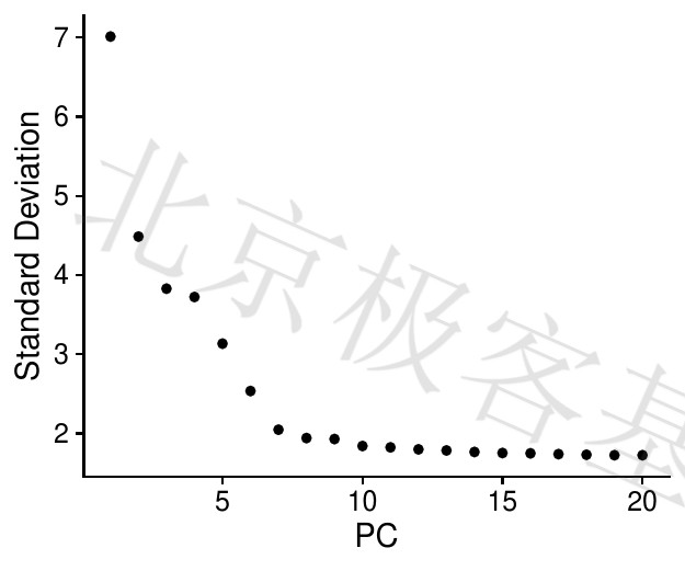
Figure 6.10: T-PCA result
PDF 文件 : T-main_pc1.jpg
图例[Figure legends]
基于每个(ElbowPlot函数)解释的方差百分比对主成分进行排序。在这个例子中,我们可以观察PC9-10周围的“肘部”,这表明大多数真实信号都是在前10PC中捕获的。
Sort the principal components based on the percentage of variance explained by each (ElbowPlot function). In this example, we can observe the “elbows” around PC9-10, which indicates that most of the real signals were captured in the top 10PCs.